
Building GPT from Scratch — Part 10: Disaggregated Inference — Splitting Prefill and Decode
TL;DR
Prefill is compute-bound (process all prompt tokens in parallel). Decode is memory-bound (read KV cache for one new token at a time). Running both on the same GPU forces a compromise — you can't optimize for both simultaneously. Disaggregated inference separates them: a prefill cluster processes prompts and ships the KV cache to a decode cluster that generates tokens. The prefill pool maximizes FLOPS utilization. The decode pool maximizes memory bandwidth utilization. Result: 2–4× higher throughput at the same latency targets, because each pool runs hardware at its natural operating point.

The Problem: Two Workloads, One GPU
In Post 6, we noted that inference has two distinct phases:
Prefill (processing the prompt):
All prompt tokens processed in parallel
Large matrix multiplications (batch of tokens × model weights)
Compute-bound: GPU arithmetic units are the bottleneck
Duration: proportional to prompt length
Decode (generating tokens):
One new token at a time
Tiny matrix multiplications (1 token × model weights)
Must read entire KV cache from memory each step
Memory-bandwidth-bound: GPU memory bus is the bottleneck
Duration: proportional to output length
These have fundamentally different hardware requirements — prefill uses 60-80% of available FLOPS with low memory bandwidth, while decode uses <5% of FLOPS but saturates memory bandwidth. They have opposite bottlenecks.
When both run on the same GPU, you get interference:
A long prefill (2000-token prompt) blocks ongoing decode requests — those users see a latency spike ("stall")
Decode requests keep the GPU memory-bound at <5% compute utilization — wasting the expensive FLOPS you're paying for
Batching decode requests helps, but a prefill interrupting the batch ruins the latency profile
You can't independently scale prefill and decode capacity
The Disaggregated Architecture
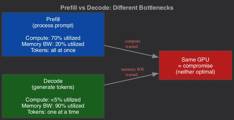
The fix: dedicated hardware pools for each phase.
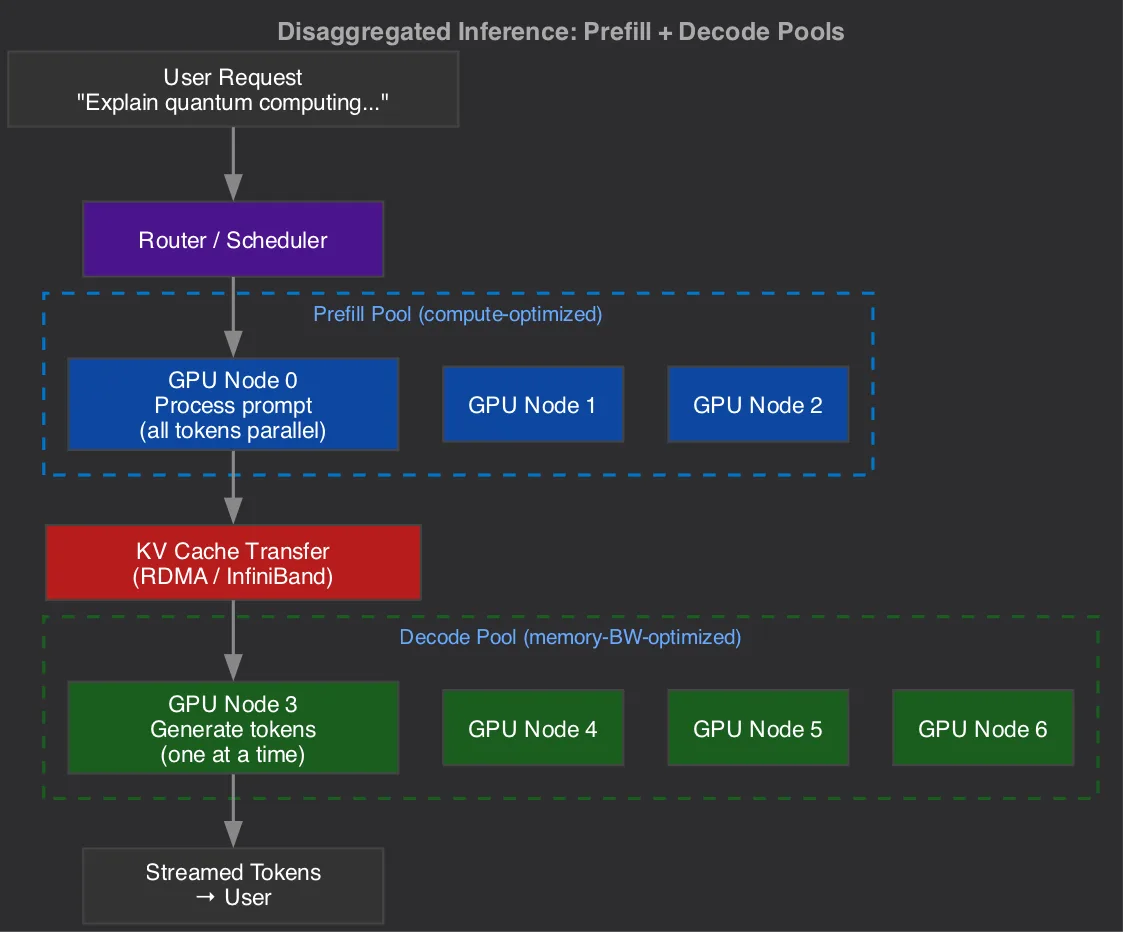
The Flow
Request arrives → router sends prompt to a prefill worker
Prefill worker processes all prompt tokens in one batched forward pass, produces KV cache
KV cache transfer → the computed KV tensors move to a decode worker
Decode worker generates tokens one at a time using the received KV cache
Tokens stream back to the user as they're generated
Why This Works: The Arithmetic Intensity Argument
Arithmetic intensity = FLOPs per byte of memory accessed. It determines whether a workload is compute-bound or memory-bound.
For a transformer layer with weight matrix W [d, d]:
Loading W from memory:
d² × sizeof(dtype)bytesCompute for batch of B tokens:
2 × B × d²FLOPs
Arithmetic intensity = (2 × B × d²) / (d² × sizeof) = 2B / sizeof

For bf16 (2 bytes):
  B=1    (single decode token): intensity = 1 FLOP/byte
  B=32   (small decode batch):  intensity = 32 FLOP/byte
  B=512  (prefill prompt):      intensity = 512 FLOP/byte
  B=2048 (long prompt):         intensity = 2048 FLOP/byte

H100 roofline:
  Peak compute: 990 TFLOPS (bf16)
  Peak memory BW: 3.35 TB/s
  Ridge point: 990/3.35 = ~295 FLOP/byte
Prefill (B=512+) operates well above the ridge point → compute-bound. The GPU arithmetic units are the bottleneck. Memory bandwidth is underutilized.
Decode (B=1 per request, even batched B=64) operates below the ridge point → memory-bandwidth-bound. The GPU spends most time waiting for weight data to arrive from HBM. Compute units are idle.
This is why mixing them wastes hardware:
During prefill: memory bus is idle → decode could be using it
During decode: compute is idle → prefill could be using it
Disaggregation lets each pool saturate its respective bottleneck
The KV Cache Transfer Problem
The critical challenge: moving KV cache from prefill to decode GPUs.
How Big Is the KV Cache?
KV cache size per request = 2 × n_layers × n_heads × seq_len × head_dim × sizeof(dtype)

For LLaMA 70B (bf16), 2048-token prompt:
  = 2 × 80 × 64 × 2048 × 128 × 2 bytes
  = 5.2 GB per request
That's 5.2 GB that needs to move from prefill GPU to decode GPU for every request. At 100 requests/second, that's 520 GB/s of KV cache traffic.
Transfer Mechanisms
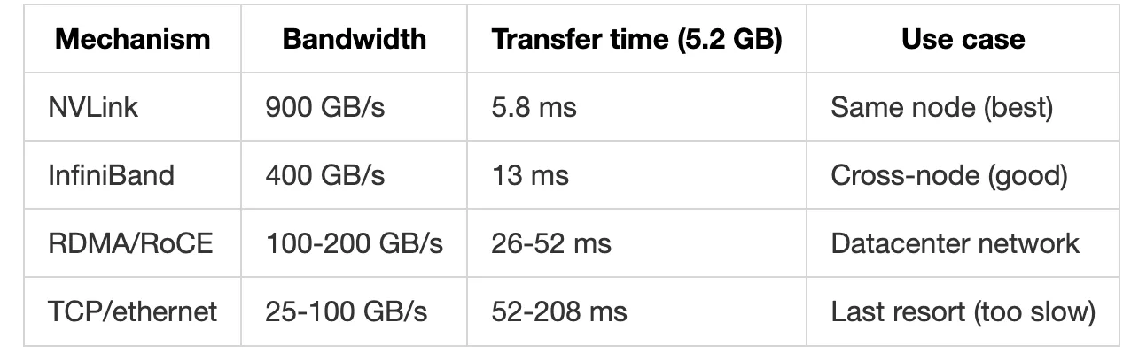
The transfer must complete before the first decode token can be generated — it directly adds to Time to First Token (TTFT). This is why same-node placement (NVLink) is strongly preferred.
Transfer Optimization: Chunked/Pipelined
Don't wait for the full KV cache. Start decoding as soon as the first layers' KV cache arrives:
Prefill GPU:  [compute layer 0][compute layer 1][compute layer 2]...
                         │                │                │
                        ▼              ▼                ▼
Transfer:     [send KV_0]     [send KV_1]     [send KV_2]...
                        │                │                │
                      ▼               ▼                ▼
Decode GPU:   [ready]         [ready]         [start decode]
                                              (layers 0-2 KV available)
By pipelining the transfer with prefill computation, the decode GPU can start generating before the prefill is even complete for later layers. This reduces TTFT significantly.
Scheduling: The Brain of the System
The router/scheduler decides:
Which prefill GPU handles each incoming request
Which decode GPU receives the KV cache
How to batch decode requests for maximum throughput
Key Scheduling Decisions
1. Prefill Batching
Group multiple incoming prompts into one prefill batch:
Request A: 500 tokens  ┐
Request B: 800 tokens  ├─ Batch together → one prefill forward pass
Request C: 300 tokens  ┘

Padded to max length (800) or use variable-length attention
This maximizes GPU utilization during prefill — a batch of 32 prompts saturates compute on an H100.
2. Decode Batching (Continuous Batching)
The decode pool uses continuous batching — new requests join the batch immediately as old ones finish:
Time →
Slot 0: [Request A decode.......][Request D decode...]
Slot 1: [Request B decode...][Request E decode........]
Slot 2: [Request C decode..........][Request F...]
                 ↑
         KV caches arrive from prefill pool at different times
         Slots are filled continuously, no waiting for a full batch
This is critical: without continuous batching, the decode pool would stall waiting to form full batches. With it, GPU memory bandwidth stays saturated.
3. Priority and SLA Routing
High-priority (interactive chat):
  → Route to low-occupancy decode GPU
  → Minimize time-to-first-token
  → Accept lower batch efficiency

Batch processing (summarization, embeddings):
  → Pack into large prefill batches
  → Route to high-occupancy decode GPU
  → Optimize for throughput, relax latency
How This Maps to Our Code
Let's trace how our existing generate.py would split across the disaggregated system:
# ORIGINAL (single-device, from Post 6):
def generate(model, tokenizer, prompt, max_new_tokens, ...):
    token_ids = tokenizer.encode(prompt)
    x = torch.tensor([token_ids], device=device)

    model.clear_cache()

    # Phase 1: Prefill — ALL on one device
    logits, _ = model(x, use_cache=True, pos_offset=0)
    next_token = sample(logits[:, -1, :])
    x = torch.cat([x, next_token], dim=1)

    # Phase 2: Decode — ALL on same device
    for i in range(1, max_new_tokens):
        logits, _ = model(x[:, -1:], use_cache=True, pos_offset=x.shape[1]-1)
        next_token = sample(logits[:, -1, :])
        x = torch.cat([x, next_token], dim=1)
# DISAGGREGATED (conceptual):
# === PREFILL WORKER (GPU pool A) ===
def prefill_worker(model, request):
token_ids = tokenizer.encode(request.prompt)
x = torch.tensor([token_ids], device=device)
model.clear_cache()
logits, _ = model(x, use_cache=True, pos_offset=0)
# Extract KV cache from model
kv_cache = extract_kv_cache(model)
first_token = sample(logits[:, -1, :])
# Send KV cache + first token to decode worker
return PrefillResult(
kv_cache=kv_cache, # the expensive artifact
first_token=first_token,
seq_len=x.shape[1],
request_id=request.id,
)
# === KV CACHE TRANSFER (network) ===
def transfer_kv_cache(prefill_result, decode_worker_addr):
# Serialize and send KV cache over RDMA/NVLink
# For LLaMA 70B, 2K context: ~5.2 GB per request
send_rdma(decode_worker_addr, prefill_result.kv_cache)
# === DECODE WORKER (GPU pool B) ===
def decode_worker(model, prefill_result, max_new_tokens):
# Load received KV cache into model
inject_kv_cache(model, prefill_result.kv_cache)
tokens = [prefill_result.first_token]
pos = prefill_result.seq_len
for i in range(max_new_tokens - 1):
x = torch.tensor([[tokens[-1]]], device=device)
logits, _ = model(x, use_cache=True, pos_offset=pos)
next_token = sample(logits[:, -1, :])
tokens.append(next_token.item())
pos += 1
yield next_token # stream to user
model.clear_cache()The model architecture is identical. The KV cache format is identical. The only difference is where each phase runs and the transfer step between them.
Extracting and Injecting KV Cache
The missing piece in our implementation — making the KV cache portable:
def extract_kv_cache(model):
    """Pull KV cache tensors out of model for transfer."""
    cache = []
    for block in model.blocks:
        cache.append({
            'k': block.attn.cache_k.clone(),  # [B, n_heads, seq_len, head_dim]
            'v': block.attn.cache_v.clone(),
        })
    return cache


def inject_kv_cache(model, cache):
    """Load KV cache into model (on decode worker after transfer)."""
    for i, block in enumerate(model.blocks):
        block.attn.cache_k = cache[i]['k'].to(device)
        block.attn.cache_v = cache[i]['v'].to(device)


def kv_cache_size_bytes(model, seq_len, dtype=torch.bfloat16):
    """Calculate KV cache size for capacity planning."""
    per_layer = 2 * model.config.n_heads * seq_len * (model.config.embed_dim // model.config.n_heads)
    total_elements = per_layer * model.config.n_layers
    bytes_per_element = 2 if dtype == torch.bfloat16 else 4
    return total_elements * bytes_per_element
Performance: Why Disaggregation Wins
The Utilization Problem (Colocated)
On a colocated system (prefill + decode on same GPU):
Timeline for one GPU handling 4 requests:

Time →
[Prefill A (50ms)][ Decode A .............................(2000ms)]
                  ↑ GPU compute utilization drops from 70% to 3%

[Prefill B][ Decode B ..........................]
[Prefill C][ Decode C ..................]
[Prefill D][ Decode D ............................]

Avg GPU compute utilization: ~10%
Avg memory BW utilization: ~60%
The GPU spends 95% of wall-clock time in decode mode, where compute utilization is <5%. You're paying for 990 TFLOPS and using 50.
The Utilization Win (Disaggregated)
PREFILL POOL (4 GPUs):
[Prefill A][Prefill E][Prefill I][Prefill M]...  ← always prefilling
[Prefill B][Prefill F][Prefill J][Prefill N]...
[Prefill C][Prefill G][Prefill K][Prefill O]...
[Prefill D][Prefill H][Prefill L][Prefill P]...

Compute utilization: 60-80% (saturated)

DECODE POOL (8 GPUs, each handling 50+ concurrent decodes):
[Decode batch of 50 requests per step]...  ← always decoding
[Decode batch of 50 requests per step]...
...

Memory BW utilization: 80-90% (saturated)
Batched decode: higher effective compute utilization too
Each pool operates at its hardware's optimal point. The prefill pool stays compute-saturated. The decode pool stays memory-bandwidth-saturated with large decode batches.
Quantitative Gains
From Splitwise (Microsoft, 2024) and DistServe (PKU, 2024):
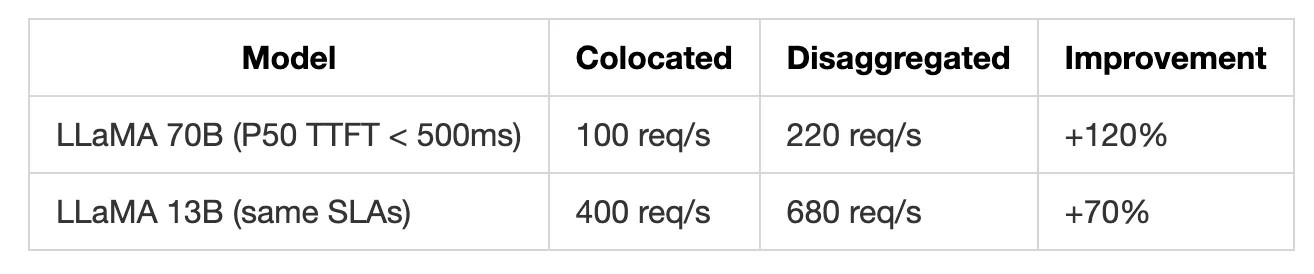
Cost efficiency: same throughput at 1.4-2× fewer GPUs.
The gains come from:
No prefill/decode interference (prefills don't stall decode batches)
Higher batch sizes in decode (more requests = better memory BW utilization)
Independent scaling (prefill-heavy workloads get more prefill GPUs)
Scaling the Pools Independently
Different workloads have different prefill:decode ratios:
Chatbot (short prompts, long responses):
  Prefill: 100 tokens, 5ms
  Decode:  500 tokens, 5000ms
  Ratio:   1:1000 (time)
  → Need many more decode GPUs than prefill

Summarization (long prompts, short responses):
  Prefill: 10000 tokens, 200ms
  Decode:  200 tokens, 2000ms
  Ratio:   1:10 (time)
  → Need relatively more prefill GPUs

Code completion (medium prompt, short response):
  Prefill: 2000 tokens, 40ms
  Decode:  50 tokens, 500ms
  Ratio:   1:12
  → Balanced
With disaggregation, you can size each pool independently:
Chatbot workload:   2 prefill GPUs + 16 decode GPUs
Summarization:      8 prefill GPUs + 8 decode GPUs
Mixed (production): autoscale based on queue depth
Colocated systems can't do this — every GPU must handle both phases, so you overprovision for the dominant phase and waste capacity for the other.
KV Cache Compression: Reducing Transfer Cost
The 5.2 GB KV cache per request is the main bottleneck. Techniques to reduce it:
1. KV Cache Quantization
# Store KV cache in int8 instead of bf16 → 2× reduction
def quantize_kv_cache(cache):
    quantized = []
    for layer in cache:
        k_scale = layer['k'].abs().max() / 127.0
        v_scale = layer['v'].abs().max() / 127.0
        quantized.append({
            'k': (layer['k'] / k_scale).to(torch.int8),
            'v': (layer['v'] / v_scale).to(torch.int8),
            'k_scale': k_scale,
            'v_scale': v_scale,
        })
    return quantized  # 2.6 GB instead of 5.2 GB
2. KV Cache Eviction (Attention Sink)
Not all KV entries are equally important. Recent work shows attention concentrates on:
The first few tokens ("attention sink")
Recent tokens (local context)
A few high-attention "landmark" tokens
def compress_kv_cache(cache, seq_len, keep_ratio=0.5):
    """Keep first 4 tokens + most recent 50% + top-attention tokens."""
    keep_start = 4  # attention sink
    keep_recent = int(seq_len * 0.4)
    # Evict middle tokens with low attention scores
    # Reduces transfer by 50% with minimal quality loss
3. Multi-Query / Grouped-Query Attention
Modern models (LLaMA 2+, Mistral) use GQA — fewer KV heads than query heads:
Standard MHA:  32 Q heads, 32 KV heads → full KV cache
GQA (LLaMA):  32 Q heads,  8 KV heads → 4× smaller KV cache

LLaMA 70B with GQA, 2048 context:
  KV cache = 2 × 80 × 8 × 2048 × 128 × 2 = 650 MB  (not 5.2 GB!)
GQA was designed partly for this reason — reducing KV cache size benefits both memory during decode AND transfer cost in disaggregated systems.
Going Multi-Node: Disaggregated Inference at Cluster Scale
Real disaggregated serving runs across dozens to hundreds of machines. The model itself is too large for one GPU, so each "worker" is actually a multi-GPU instance using tensor parallelism internally. The cluster orchestrates a fleet of these instances.
The Full Architecture
The cluster has a load balancer/router at the top that handles request admission, SLA-aware routing, and queue depth monitoring. It routes requests to either the prefill pool (compute-optimized nodes) or the decode pool (memory-optimized nodes), with KV cache transfer over RDMA/InfiniBand connecting the two pools.
For LLaMA 70B serving:
Each instance uses 8 GPUs with tensor parallelism (model sharded across 8 GPUs)
Prefill pool: 3 nodes (24 GPUs) — handles ~200 prefill requests/sec
Decode pool: 8 nodes (64 GPUs) — handles ~800 concurrent decode streams
Total: 88 GPUs serving thousands of users concurrently
KV Cache Transfer Over the Network
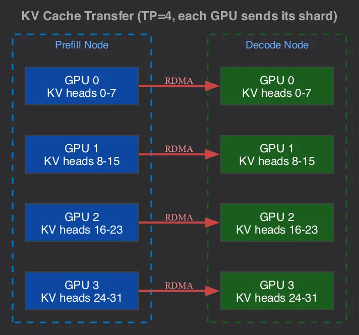
The critical data path: prefill node → network → decode node.
# Prefill worker (Node 0, 8 GPUs with TP=8)
# Each GPU holds 1/8 of the KV cache (split by heads)

def prefill_and_transfer(request, decode_node_addr):
    # Prefill happens across 8 GPUs (tensor parallel)
    logits = model.forward(request.tokens)  # TP handles the distribution

    # Each GPU extracts its local KV cache shard
    local_kv = extract_local_kv_cache(model)  # 1/8 of full cache

    # Transfer: each GPU sends its shard to the corresponding GPU
    # on the decode node (GPU 0 → GPU 0, GPU 1 → GPU 1, etc.)
    # This is a point-to-point RDMA transfer, NOT a collective
    rdma_send(
        dest=f"{decode_node_addr}:gpu{local_rank}",
        data=local_kv,
    )
# Decode worker (Node 5, 8 GPUs with TP=8)
def receive_and_decode(source_node_addr, request):
# Each GPU receives its KV cache shard from the corresponding
# prefill GPU (point-to-point)
local_kv = rdma_recv(source=f"{source_node_addr}:gpu{local_rank}")
inject_local_kv_cache(model, local_kv)
# Decode proceeds with tensor parallelism as normal
for step in range(max_tokens):
logits = model.forward(last_token) # TP handles distribution
token = sample(logits)
yield tokenKey insight: the KV cache is already sharded by heads due to tensor parallelism. Transfer is embarrassingly parallel — each GPU pair communicates independently. With 8 GPUs: 8 parallel RDMA transfers of 1/8 the data each.
Transfer for LLaMA 70B (GQA), 4096 context, TP=8:
  Full KV cache: 2 × 80 layers × 8 KV_heads × 4096 × 128 × 2 bytes = 1.3 GB
  Per-GPU shard: 1.3 GB / 8 = 162 MB
  Over InfiniBand (400 GB/s): 0.4ms per GPU (all 8 in parallel)
  Total transfer time: 0.4ms  ← negligible
The Scheduler: Multi-Node Coordination
The scheduler is the brain. For each incoming request, it makes four decisions:
Which prefill node? Pick the one with the shortest queue — minimizes wait time.
Which decode node? Pick one with enough free KV cache memory to hold this request through its full generation. A 4096-token request needs ~162 MB of KV cache space (for LLaMA 70B with GQA and TP=8).
Placement affinity? Prefer a prefill/decode pair in the same rack — the KV cache transfer is faster (0.1ms vs 0.5ms+ across racks).
Reserve before computing. The scheduler reserves a decode slot before starting the prefill. Otherwise you might compute a KV cache with nowhere to send it — wasting prefill compute and blocking the user.
When a request finishes generating, the scheduler releases its KV cache memory on the decode node, making room for the next request. This is the core resource lifecycle: reserve → prefill → transfer → decode → release.
Memory Management on Decode Nodes
The decode pool's scarce resource is HBM for KV caches. Each decode GPU must hold:
Model parameters (sharded via TP): fixed
KV caches for all active requests: variable, grows with concurrency
H100 80GB, LLaMA 70B (TP=8):
  Model params per GPU:     ~10 GB (70B / 8, in bf16)
  Available for KV caches:  ~70 GB
  KV cache per request (4K context, GQA): 162 MB per GPU
  Max concurrent requests:  70 GB / 162 MB ≈ 430 requests per GPU

  Decode batch: up to 430 concurrent generations per node
This is why decode nodes can batch hundreds of requests — each request's KV cache is relatively small (especially with GQA). The large batch size makes decode more compute-efficient (higher arithmetic intensity), partially recovering from the memory-bound regime.
PagedAttention (vLLM's approach): allocates KV cache in fixed-size blocks, just like how an OS manages virtual memory with pages. Without it, you'd pre-allocate the maximum possible KV cache for every request (like malloc(max_seq_len) upfront) — wasting memory on requests that finish early. With paging, memory is allocated in small blocks as needed and freed immediately when a request completes. Same idea as virtual memory: avoid fragmentation, improve utilization, decouple allocation from physical layout.
Autoscaling the Pools
The two pools scale on different signals:
Prefill pool scales on: queue depth (requests waiting for prefill)
  → High queue depth = users waiting for TTFT = add prefill capacity
  → Low queue depth = prefill nodes underutilized = scale down

Decode pool scales on: KV cache memory utilization
  → High memory usage = can't accept new requests = add decode capacity
  → Low memory usage = decode nodes have room = scale down
This is the operational advantage: a spike in long-prompt traffic (e.g., document summarization surge) adds prefill nodes without touching decode. A spike in concurrent users (many active chats) adds decode nodes without touching prefill. Colocated systems can't do this — they'd have to scale both capabilities together, wasting whichever isn't the bottleneck.
Network Topology Matters
BEST: Prefill and decode nodes in same rack
  → NVSwitch or short InfiniBand hop
  → <0.2ms KV transfer
  → Works like intra-node

GOOD: Same datacenter, leaf-spine fabric
  → 1-2 InfiniBand hops
  → 0.5-2ms KV transfer
  → Acceptable for most SLAs

BAD: Cross-datacenter or over ethernet
  → 5-50ms KV transfer
  → May exceed TTFT budget
  → Only viable for batch/async workloads
Production deployments co-locate prefill and decode pools in the same InfiniBand fabric. Some systems (Mooncake) place them in the same rack and use NVSwitch for near-zero transfer overhead.
Heterogeneous Hardware
A key advantage of disaggregation: different GPU types for different roles.
Prefill pool: H100 SXM (highest FLOPS, 990 TF bf16)
  → Maximizes prompt processing speed
  → Expensive per GPU but each handles many requests/sec

Decode pool: A100 or L40S (lower cost, still good memory BW)
  → Memory bandwidth is the bottleneck anyway
  → H100's extra FLOPS are wasted during decode
  → 2× more GPUs at same budget → 2× more concurrent requests

Cost savings: H100 ($30K) vs A100 ($15K)
  Decode doesn't need H100's compute → use A100 for decode
  Same throughput, ~30% lower infrastructure cost
This is the Splitwise paper's core insight: you don't need the same GPU everywhere.
Production Systems Using This
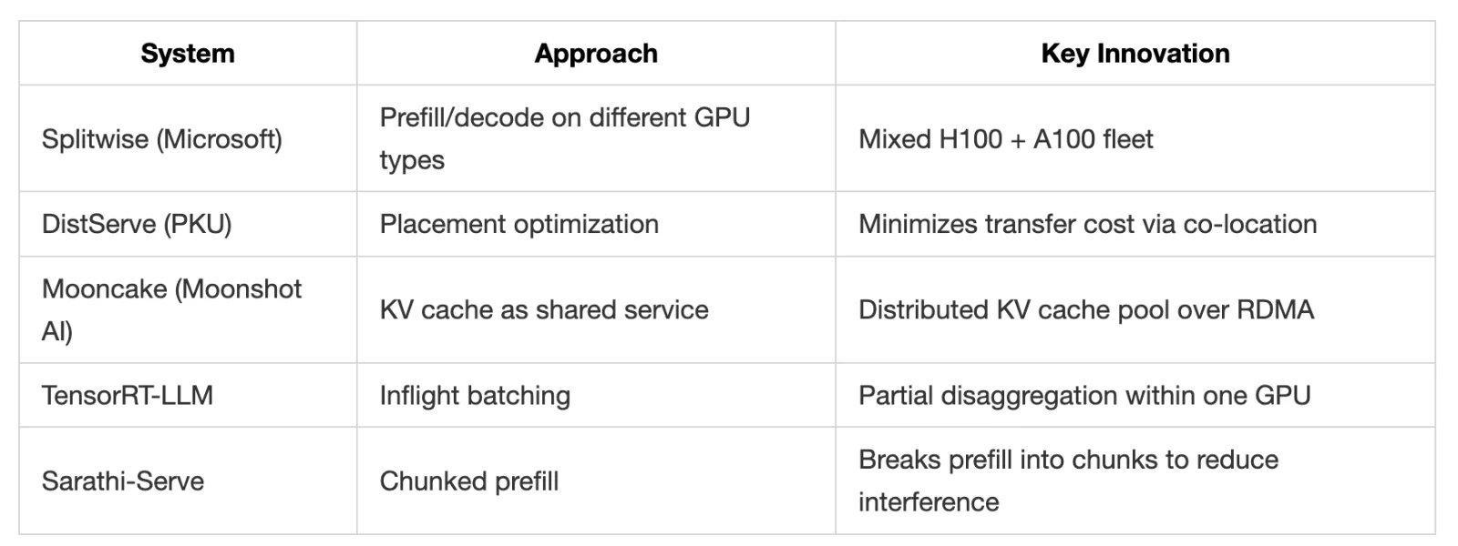
The trend is clear: every major serving system is moving toward some form of prefill/decode separation.
Running on a MacBook (Simulated)
True disaggregation needs multiple GPUs. But you can simulate the architecture on a MacBook to understand the flow:
# Simulate disaggregated inference with separate model instances
# (both on the same device, but demonstrates the protocol)

def simulate_disaggregated(prompt, max_new_tokens):
    # "Prefill worker" — could be on GPU A
    prefill_model = load_model("checkpoint.pt", device)
    prefill_model.clear_cache()

    x = torch.tensor([tokenizer.encode(prompt)], device=device)
    logits, _ = prefill_model(x, use_cache=True, pos_offset=0)

    # Extract KV cache (this would be transferred over network)
    kv_cache = extract_kv_cache(prefill_model)
    first_token = sample(logits[:, -1, :])
    seq_len = x.shape[1]

    del prefill_model  # free memory (simulates separate GPU)

    # "Decode worker" — could be on GPU B
    decode_model = load_model("checkpoint.pt", device)
    inject_kv_cache(decode_model, kv_cache)

    # Decode loop
    tokens = [first_token.item()]
    for i in range(max_new_tokens - 1):
        x = torch.tensor([[tokens[-1]]], device=device)
        logits, _ = decode_model(x, use_cache=True, pos_offset=seq_len + i)
        tokens.append(sample(logits[:, -1, :]).item())

    decode_model.clear_cache()
    return tokenizer.decode(tokens)
This proves the protocol works — KV cache is portable between model instances. On real hardware, the two models would be on different GPUs with a network transfer in between.
Key Takeaways
Prefill and decode are different beasts. Prefill saturates compute (high arithmetic intensity). Decode saturates memory bandwidth (low arithmetic intensity). Mixing them on one GPU wastes both.
KV cache is the handoff artifact. The entire state of a generation is encoded in the KV cache. Transfer it, and any GPU can continue decoding. This is what makes disaggregation possible.
The transfer cost is real but manageable. LLaMA 70B's KV cache is 650 MB–5.2 GB per request (depending on GQA). Over NVLink/InfiniBand, that's 5–13ms — well within latency budgets. Quantization and GQA reduce it further.
Independent scaling is the operational win. Chatbots need more decode capacity. Summarizers need more prefill. Disaggregation lets you right-size each pool instead of overprovisioning a monolithic fleet.
This is where LLM serving is heading. Splitwise, DistServe, Mooncake — every 2024-2025 serving paper converges on this architecture. If you're building or operating LLM infrastructure, disaggregation is the next step after continuous batching.
Series Complete: From Laptop to Production Fleet
Post 1-6:  Build GPT, train it, run it — all on a MacBook
Post 7:    DDP — same code, N× throughput with multiple GPUs
Post 8:    FSDP — shard memory when model won't fit
Post 9:    Tensor Parallel — split layers for the largest models
Post 10:   Disaggregated Inference — separate prefill and decode for efficient serving
Same architecture. Same math. Different scale — from python train.py on a MacBook to 4,096 GPUs across 512 machines.