
Building GPT from Scratch — Part 3: The Transformer Architecture
TL;DR
The GPT architecture is a stack of transformer blocks, each containing causal self-attention (lets each token attend to all previous tokens) and a feed-forward network (per-token nonlinear processing). The causal mask — a single triangular matrix — is what makes it "decoder-only" and enables left-to-right generation. Residual connections enable depth; LayerNorm enables stability; multi-head attention enables tracking multiple relationships in parallel. The entire model is ~200 lines of Python.
The Problem
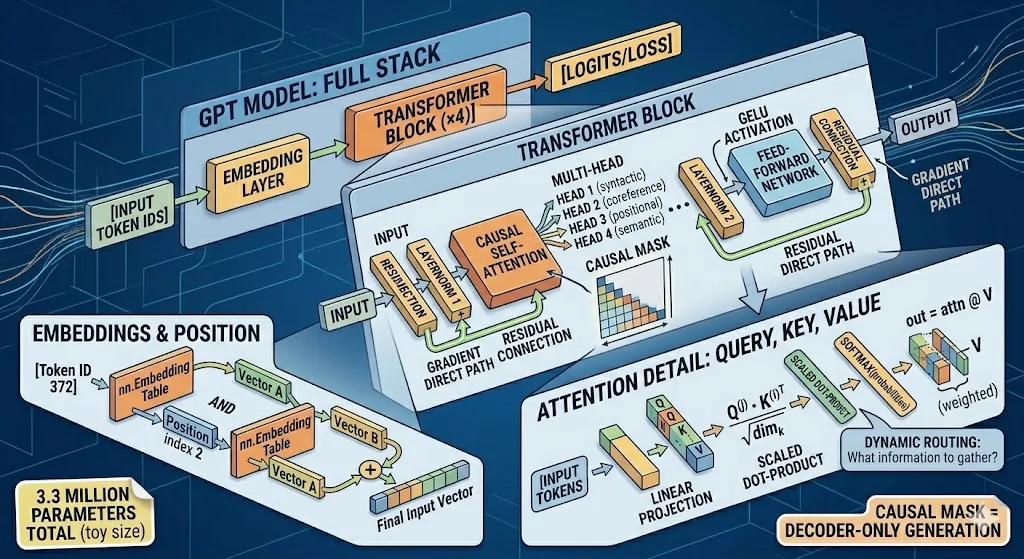
We have a sequence of token IDs. We need a function that takes those IDs and outputs a probability distribution over what token comes next. The transformer is that function.
The challenge: language has long-range dependencies. The word "it" in sentence 50 might refer to something mentioned in sentence 3. The model needs a mechanism to let any token attend to any previous token — regardless of distance. This is what self-attention provides.
The Big Picture
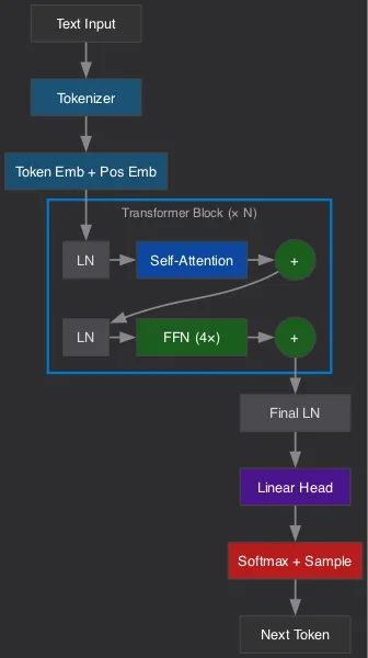
Our GPT model has 5 main components, stacked in order:
Let's build each one.
Step 1: Embeddings — Giving Tokens Meaning
A token ID like 372 is meaningless to a neural network. We need to map it to a dense vector that the model can learn with. This is what embedding layers do.
self.token_emb = nn.Embedding(vocab_size, embed_dim)    # 512 × 256
self.pos_emb = nn.Embedding(context_length, embed_dim)  # 128 × 256
Token embedding: a lookup table. Token 372 → row 372 of a [vocab_size × embed_dim] matrix. Each row is initialized randomly and trained via backpropagation. After training, tokens with similar meanings end up with similar vectors.
Position embedding: transformers process all tokens in parallel (unlike RNNs which go left-to-right). Without position information, "the cat sat on the mat" and "mat the on sat cat the" would produce identical representations. Position embedding adds a learnable vector for each position (0, 1, 2, ...) so the model knows token order.
def forward(self, idx):
    B, T = idx.shape

    # Position indices: [0, 1, 2, ..., T-1]
    pos = torch.arange(0, T, device=idx.device).unsqueeze(0)

    # Look up embeddings and add them together
    tok_emb = self.token_emb(idx)   # [B, T, embed_dim]
    pos_emb = self.pos_emb(pos)     # [1, T, embed_dim] — broadcasts over batch
    x = tok_emb + pos_emb           # [B, T, embed_dim]
Why addition and not concatenation? Concatenation would double the dimension (wasting half the model's capacity on position info). Addition works because the model learns to use orthogonal subspaces for positional and semantic information — they don't interfere much in practice.
Step 2: Causal Self-Attention — The Core Mechanism
This is the heart of the transformer. Self-attention lets each token look at every previous token and decide which ones are relevant for predicting the next word.
The Intuition
Think of reading a sentence:
"The cat, who was very old and tired, finally sat on the mat."
When processing "sat", the model needs to know:
WHO sat? → attend to "cat" (far away)
Ignore the relative clause → low attention to "who was very old and tired"
Self-attention computes this relevance dynamically for every token pair.
Query, Key, Value
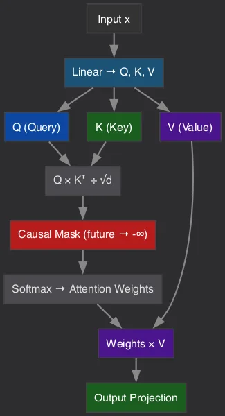
The mechanism uses three projections of the same input:
Query (Q): "What am I looking for?" — what information this token needs
Key (K): "What do I contain?" — what information this token offers
Value (V): "What do I actually provide?" — the content to pass forward if selected
# Single linear layer produces all three: Q, K, V
self.qkv = nn.Linear(embed_dim, 3 * embed_dim)

# Split into Q, K, V
qkv = self.qkv(x)                    # [B, T, 3 * embed_dim]
q, k, v = qkv.split(embed_dim, dim=-1)  # each [B, T, embed_dim]
Why one combined linear layer? Efficiency. Three separate layers would do the same math but with three separate matrix multiplications. One combined layer followed by a split is faster on GPUs.
Computing Attention Scores
# Reshape for multi-head: [B, T, embed_dim] → [B, n_heads, T, head_dim]
q = q.view(B, T, n_heads, head_dim).transpose(1, 2)
k = k.view(B, T, n_heads, head_dim).transpose(1, 2)
v = v.view(B, T, n_heads, head_dim).transpose(1, 2)

# Dot product between queries and keys
# Each q[i] asks: "how relevant is k[j] to me?"
attn = (q @ k.transpose(-2, -1)) * (head_dim ** -0.5)
Why scale by 1/√(head_dim)? Without scaling, the dot products grow with dimension size. Large dot products push softmax into regions where gradients are tiny (near 0 or 1), making learning slow. Scaling keeps the variance stable regardless of dimension.
The Causal Mask — What Makes It "Decoder-Only"
# Lower-triangular matrix: 1s below diagonal, 0s above
mask = torch.tril(torch.ones(context_length, context_length))

# Example for seq_len=5:
# [[1, 0, 0, 0, 0],   ← token 0 sees only itself
#  [1, 1, 0, 0, 0],   ← token 1 sees tokens 0-1
#  [1, 1, 1, 0, 0],   ← token 2 sees tokens 0-2
#  [1, 1, 1, 1, 0],   ← token 3 sees tokens 0-3
#  [1, 1, 1, 1, 1]]   ← token 4 sees all previous

# Set masked positions to -infinity (softmax → 0 probability)
attn = attn.masked_fill(mask[:T, :T] == 0, float("-inf"))
This is the critical constraint. By masking future tokens, we guarantee:
The model can never "cheat" by looking ahead during training
Each position's prediction depends only on past context
The model can generate text left-to-right at inference time
Without this mask, it's a BERT-style encoder (bidirectional). With it, it's GPT (autoregressive).
Softmax and Output
# Convert scores to probabilities (each row sums to 1)
attn = F.softmax(attn, dim=-1)
attn = self.attn_dropout(attn)

# Weighted sum of values — high-attention tokens contribute more
out = attn @ v  # [B, n_heads, T, head_dim]

# Reshape back: [B, n_heads, T, head_dim] → [B, T, embed_dim]
out = out.transpose(1, 2).contiguous().view(B, T, embed_dim)

# Final projection
return self.out_proj(out)
Multi-Head Attention — Why Multiple Heads?
Instead of one big attention computation, we split into N smaller ones (heads), each operating on embed_dim / n_heads dimensions.
Why? Different heads learn different patterns:
Head 1 might learn syntactic relationships (subject-verb agreement)
Head 2 might learn coreference ("she" → "Alice")
Head 3 might learn positional patterns (adjacent words)
Head 4 might learn semantic similarity
With one head, these patterns would interfere. Multiple heads let the model track multiple relationships simultaneously, then combine them via the output projection.
embed_dim = 256, n_heads = 4 → head_dim = 64
Each head: [B, T, 64] — smaller but independent attention patterns
Combined: [B, T, 256] — all patterns merged
Step 3: Feed-Forward Network — Per-Token Processing
After attention gathers context from other tokens, the feed-forward network processes each token independently:
class FeedForward(nn.Module):
    def __init__(self, config):
        self.fc1 = nn.Linear(embed_dim, 4 * embed_dim)   # expand
        self.fc2 = nn.Linear(4 * embed_dim, embed_dim)   # compress back
        self.dropout = nn.Dropout(dropout)

    def forward(self, x):
        x = F.gelu(self.fc1(x))   # expand to 4× and apply nonlinearity
        return self.dropout(self.fc2(x))  # compress back
Why 4× expansion? This is a design choice from the original transformer paper. The expansion creates a higher-dimensional space where the network can compute more complex functions, then projects back down. Think of it as: attention decides what information to gather; feed-forward decides what to do with it.
Why GELU instead of ReLU? GELU (Gaussian Error Linear Unit) is smoother than ReLU — it doesn't have a hard zero cutoff. This gives better gradients and slightly better performance in practice. GPT-2 used GELU; it's now standard.
Where do the parameters live? In a typical transformer, ~2/3 of all parameters are in the feed-forward layers. Attention is parameter-efficient (just projections); the feed-forward network is where the model stores "knowledge."
Step 4: The Transformer Block — Putting It Together
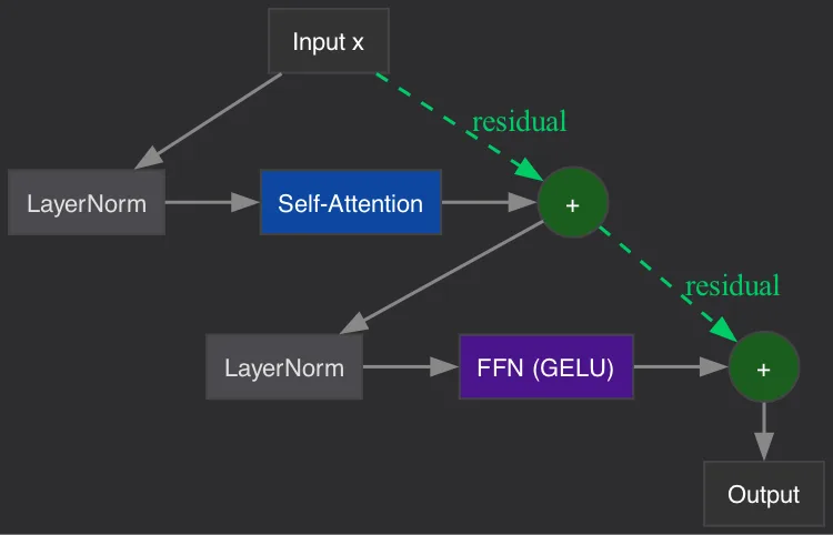
A single transformer block combines attention and feed-forward with residual connections and layer normalization:
class TransformerBlock(nn.Module):
    def __init__(self, config):
        self.ln1 = nn.LayerNorm(embed_dim)
        self.attn = CausalSelfAttention(config)
        self.ln2 = nn.LayerNorm(embed_dim)
        self.ff = FeedForward(config)

    def forward(self, x):
        x = x + self.attn(self.ln1(x))   # attention + residual
        x = x + self.ff(self.ln2(x))     # feedforward + residual
        return x
Residual Connections: Why x + f(x) Instead of Just f(x)?
Without residuals, a 6-layer network means information must pass through 6 transformations in series. Gradients vanish or explode. Training becomes unstable.
With residuals, each layer only needs to learn the delta — what to add to the current representation. If a layer has nothing useful to contribute, it can output near-zero and the input passes through unchanged. This makes deep networks trainable.
Without residuals: x → f₁ → f₂ → f₃ → f₄ (gradients must flow through all)
With residuals:    x → x + f₁(x) → x + f₁(x) + f₂(...) → ... (gradient has direct path)
LayerNorm: Why Normalize?
# Normalizes each token's vector to mean=0, variance=1
# Then applies learned scale (γ) and shift (β)
self.ln1 = nn.LayerNorm(embed_dim)
Training neural networks is sensitive to the scale of activations. If some layers produce values in [0, 1] and others in [-1000, 1000], the learning rate that works for one destroys the other. LayerNorm keeps everything on a consistent scale.
Pre-norm vs post-norm: We use pre-norm (normalize before attention/FF), which is what GPT-2 and most modern models use. The original transformer paper used post-norm. Pre-norm is more stable for training.
Step 5: The Full GPT Model
Stack everything together:
class GPT(nn.Module):
    def __init__(self, config):
        # Embeddings
        self.token_emb = nn.Embedding(config.vocab_size, config.embed_dim)
        self.pos_emb = nn.Embedding(config.context_length, config.embed_dim)
        self.drop = nn.Dropout(config.dropout)

        # N transformer blocks
        self.blocks = nn.Sequential(
            *[TransformerBlock(config) for _ in range(config.n_layers)]
        )

        # Output
        self.ln_final = nn.LayerNorm(config.embed_dim)
        self.head = nn.Linear(config.embed_dim, config.vocab_size, bias=False)

        # Weight tying: output projection shares weights with token embedding
        self.token_emb.weight = self.head.weight
Weight Tying: Why Share Embedding and Output Weights?
The token embedding maps: token ID → vector. The output head maps: vector → token ID probabilities.
These are inverse operations. By sharing the weight matrix, we:
Reduce parameter count (no duplicate matrix)
Enforce consistency: if two tokens have similar embeddings, they'll have similar output probabilities
Improve training: both the input and output side contribute gradients to the same matrix
This is standard practice in language models since 2016.
Weight Initialization
def _init_weights(self, module):
    if isinstance(module, nn.Linear):
        torch.nn.init.normal_(module.weight, mean=0.0, std=0.02)
        if module.bias is not None:
            torch.nn.init.zeros_(module.bias)
    elif isinstance(module, nn.Embedding):
        torch.nn.init.normal_(module.weight, mean=0.0, std=0.02)
Why std=0.02? At initialization, we want activations to have reasonable magnitude. Too large → exploding gradients. Too small → dead neurons. 0.02 keeps the initial forward pass well-behaved for typical model sizes. GPT-2 used this value.
The Forward Pass — End to End
def forward(self, idx, targets=None):
    B, T = idx.shape

    # 1. Embeddings: token IDs → dense vectors with position info
    pos = torch.arange(0, T, device=idx.device).unsqueeze(0)
    x = self.drop(self.token_emb(idx) + self.pos_emb(pos))

    # 2. Transformer blocks: build contextual representations
    for block in self.blocks:
        x = block(x)

    # 3. Output: project to vocabulary probabilities
    x = self.ln_final(x)
    logits = self.head(x)  # [B, T, vocab_size]

    # 4. Loss (during training): compare predictions to actual next tokens
    loss = None
    if targets is not None:
        loss = F.cross_entropy(
            logits.view(-1, logits.size(-1)),  # flatten to [B*T, vocab_size]
            targets.view(-1),                   # flatten to [B*T]
        )

    return logits, loss
Every position simultaneously predicts its next token. At position 3, the model outputs a probability distribution over all 512 tokens — its best guess for what token 4 should be. During training, we know the answer and compute the loss. During generation, we sample from this distribution.
Our Model's Configuration
config = Config(
    vocab_size=512,        # number of tokens our BPE tokenizer produces
    context_length=128,    # max sequence length (tokens)
    n_layers=4,            # transformer blocks stacked
    n_heads=4,             # parallel attention heads
    embed_dim=256,         # dimension of all internal representations
    dropout=0.1,           # regularization
)
This gives us 3.3 million parameters. For reference:
GPT-2 small: 124M parameters
GPT-3: 175B parameters
Our model: 3.3M parameters
Same architecture. Different scale. The mechanism is identical.
Parameter Breakdown
Where do the 3.3M parameters actually live?
Token embedding:      512 × 256 =     131,072  (shared with output head)
Position embedding:   128 × 256 =      32,768
Per transformer block:
  QKV projection:     256 × 768 =     196,608
  Output projection:  256 × 256 =      65,536
  FF layer 1:         256 × 1024 =    262,144
  FF layer 2:         1024 × 256 =    262,144
  LayerNorms (×2):    256 × 2 × 2 =     1,024
  Subtotal per block:                  787,456
× 4 blocks:                          3,149,824
Final LayerNorm:      256 × 2 =            512
─────────────────────────────────────────────
Total:                              ~3,314,000
Most parameters (~95%) are in the transformer blocks. Of those, ~67% are in the feed-forward layers. Attention itself is relatively cheap in parameters — its cost is in compute (the O(n²) matrix multiplication).
Key Takeaways
Self-attention is dynamic routing. Unlike convolutions (fixed receptive field) or RNNs (sequential bottleneck), attention lets any token attend to any previous token directly. The relevance is learned, not hardcoded.
The causal mask is what makes it generative. One line of code —
masked_fill(mask == 0, -inf)— is the difference between GPT (generates) and BERT (classifies).Residual connections enable depth. Without them, you can't stack more than a few layers before training collapses.
The architecture is simple. The same 5 components (embed, attend, feedforward, normalize, project) repeated N times. Power comes from scale, not complexity.
Full code: github.com/the-last-programmers/gpt-from-scratch
Next: pretraining — teaching this architecture to predict the next token.