
Building GPT from Scratch — Part 4: Pretraining
TL;DR
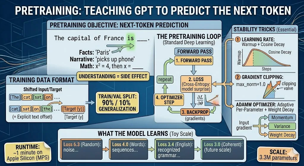
Pretraining has one objective: predict the next token. That's it. No grammar rules, no world knowledge injected — just next-token prediction via cross-entropy loss. To predict well, the model must learn language structure, facts, and reasoning as side effects. Training stability comes from three tricks: learning rate warmup + cosine decay, gradient clipping at 1.0, and AdamW optimizer with weight decay. Our 3.3M model trains in ~1 minute on a MacBook, dropping loss from 6.3 (random) to 3.4 (basic English).
The Problem
We have a transformer architecture with 3.3 million randomly initialized parameters. Right now, it outputs random noise. We need to find parameter values that make it produce coherent English.
The question: what objective do we train on?
The answer — and this is perhaps the most surprising fact about modern AI — is incredibly simple: predict the next token.
That's it. No grammar rules. No world knowledge. No explicit reasoning capability. Just: given tokens [0...t], predict token [t+1]. Everything else (grammar, facts, reasoning, creativity) emerges as a side effect of getting good at this one task.
Why Next-Token Prediction Works
This is counterintuitive. How does "autocomplete on steroids" produce intelligence?
The key insight: to predict the next token well, you must understand the text.
Consider predicting the next word in:
"The capital of France is ___"
To get this right, the model must have learned the fact that France's capital is Paris. It needs world knowledge.
"She picked up the phone and ___"
The model must understand causality, common actions, narrative structure.
"If x² = 4, then x = ___"
The model must have learned mathematical reasoning.
The prediction objective forces the model to build internal representations of grammar, facts, logic, and reasoning — because those representations help it predict better. It's learning to compress the training data, and compression requires understanding.
This is sometimes called the "compression hypothesis": a sufficiently good predictor must be a good world model.
The Training Setup
Data Format
Training data is simply text, split into chunks of context_length tokens:
class TextDataset:
    def __init__(self, token_ids, context_length):
        self.token_ids = torch.tensor(token_ids, dtype=torch.long)
        self.context_length = context_length

    def __getitem__(self, idx):
        start = idx * self.context_length
        end = start + self.context_length

        x = self.token_ids[start:end]       # input
        y = self.token_ids[start + 1:end + 1]  # target (shifted by 1)
        return x, y
The target is the input shifted by one position:
Input:  [The] [cat] [sat] [on] [the] [mat]
Target: [cat] [sat] [on]  [the] [mat] [.]
Every position simultaneously tries to predict its next token. A single training example of 128 tokens gives us 128 prediction tasks at once.
The Loss Function: Cross-Entropy
loss = F.cross_entropy(
    logits.view(-1, vocab_size),   # model's predictions: [B*T, vocab_size]
    targets.view(-1),               # actual next tokens:  [B*T]
)
Cross-entropy measures: "how surprised was the model by the actual next token?"
If the model assigns 90% probability to the correct token → loss ≈ 0.1 (good)
If the model assigns 1% probability to the correct token → loss ≈ 4.6 (bad)
Random chance (uniform over 512 tokens) → loss ≈ 6.2 (untrained model)
Our goal: drive the loss from 6.2 (random) toward as low as possible.
The Training Loop
model.train()
for step in range(max_steps):
    # 1. Get a batch of training data
    x, y = get_batch(train_dataset, batch_size, device)

    # 2. Forward pass: compute predictions and loss
    logits, loss = model(x, y)

    # 3. Backward pass: compute gradients
    loss.backward()

    # 4. Clip gradients (prevent explosion)
    torch.nn.utils.clip_grad_norm_(model.parameters(), 1.0)

    # 5. Update parameters
    optimizer.step()

    # 6. Reset gradients for next step
    optimizer.zero_grad()
Each step:
Grab a random chunk of text from the corpus
Run it through the model, get the loss
Backpropagation computes ∂loss/∂parameter for every parameter
The optimizer uses those gradients to nudge parameters toward lower loss
Repeat
Let's examine each critical component.
The Optimizer: AdamW
optimizer = torch.optim.AdamW(
    model.parameters(),
    lr=3e-4,           # peak learning rate
    weight_decay=0.1,  # L2 regularization
)
Why AdamW and not plain SGD?
SGD (Stochastic Gradient Descent): one learning rate for all parameters. If gradient is 0.001 for one parameter and 1000 for another, one of them gets a terrible update.
Adam (Adaptive Moment Estimation): maintains a per-parameter learning rate. Tracks both the gradient mean (momentum) and gradient variance. Parameters with consistently large gradients get smaller updates; parameters with small, noisy gradients get larger updates.
AdamW = Adam + decoupled weight decay. Weight decay (multiplying all weights by 0.999 each step) is a form of regularization that prevents weights from growing too large. AdamW implements this correctly (plain Adam's weight decay interacts poorly with the adaptive learning rate).
Every modern LLM uses AdamW.
Learning Rate Schedule
The learning rate isn't constant. It follows a warmup + cosine decay schedule:
def get_lr(step):
    # Phase 1: Linear warmup (first 100 steps)
    if step < warmup_steps:
        return (step + 1) / warmup_steps

    # Phase 2: Cosine decay to zero
    progress = (step - warmup_steps) / (max_steps - warmup_steps)
    return 0.5 * (1 + math.cos(math.pi * progress))
Visualized:
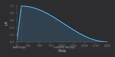
Why warmup? At initialization, the model's representations are random. Large learning rates push parameters far based on meaningless gradients. Warmup lets the model "settle" into a reasonable region before applying full learning rate.
Why cosine decay? As training progresses, the model is closer to optimal. Smaller updates prevent overshooting. Cosine gives a smooth decay that doesn't drop too fast (like exponential) or stay too high (like constant).
Gradient Clipping
grad_norm = torch.nn.utils.clip_grad_norm_(model.parameters(), max_norm=1.0)Occasionally, a batch produces unusually large gradients (a "gradient spike"). Without clipping, one bad batch can destroy hours of training progress by sending parameters to extreme values.
Gradient clipping scales the entire gradient vector so its norm never exceeds 1.0. It preserves the gradient direction but limits its magnitude. This is essential for stable training.
Gradient Accumulation
for micro_step in range(grad_accum_steps):
    x, y = get_batch(train_dataset, batch_size, device)
    logits, loss = model(x, y)
    loss = loss / grad_accum_steps  # normalize
    loss.backward()                 # accumulate gradients

# Only update after all micro-steps
optimizer.step()
optimizer.zero_grad()
The problem: we want a large effective batch size (more stable gradients), but our GPU/memory can only fit a small batch.
The solution: accumulate gradients over multiple forward passes, then do one update. With batch_size=16 and grad_accum_steps=4, the effective batch size is 64 — but we never hold more than 16 samples in memory.
This is how people train large models on limited hardware.
Training/Validation Split
split = int(len(tok   en_ids) * 0.9)
train_dataset = TextDataset(token_ids[:split], context_length)
val_dataset = TextDataset(token_ids[split:], context_length)
We hold out 10% of the data for validation. The model never trains on this data — it's used to measure generalization.
If training loss drops but validation loss doesn't → the model is memorizing, not learning. If both drop together → the model is learning genuine patterns.
step     0 | train loss 6.2926 | val loss 6.3042  ← random (correct for 512 vocab)
step   100 | train loss 4.7071 | val loss 4.7251  ← learning fast
step   200 | train loss 4.2015 | val loss 4.1096  ← still improving
step   300 | train loss 4.0547 | val loss 3.9854  ← diminishing returns
step   400 | train loss 4.0264 | val loss 3.9230  ← converging
The starting loss (6.29) is close to ln(512) = 6.24 — the theoretical loss for uniform random predictions over 512 tokens. This confirms our model is correctly initialized (not biased toward any token).
Running on Apple Silicon (MPS)
def get_device():
    if torch.backends.mps.is_available():
        return torch.device("mps")
    elif torch.cuda.is_available():
        return torch.device("cuda")
    return torch.device("cpu")
Apple's Metal Performance Shaders (MPS) backend lets PyTorch use the GPU on Apple Silicon Macs. For our 3.3M model:
CPU: ~50 steps/sec
MPS: ~200 steps/sec (4× faster)
CUDA (NVIDIA): would be faster still, but we don't need it at this scale
The entire training (2000 steps) completes in ~1 minute on an M-series Mac.
What the Model Learns
After 2000 steps, the loss drops from 6.3 to ~3.4. What does this mean in practice?
Loss 6.3 → random noise, no English structure
Loss 5.0 → learns common character patterns (th, er, ing)
Loss 4.0 → produces word-like sequences, some real words
Loss 3.5 → mostly recognizable English, some grammar
Loss 3.0 → (would need more data/parameters) coherent sentences
Our model at loss 3.4 outputs:
Input: "The "
Output: "The quengerigned and profection, Tweenerved by the mary off"
Not coherent — but recognizably English. Real words mixed with plausible-looking fake ones. Grammar partially correct. With more data and more parameters, this becomes fluent text.
Key Takeaways
The objective is absurdly simple. Predict the next token. No hand-crafted rules, no linguistic knowledge, no explicit reasoning training. Understanding emerges from prediction.
The training loop is standard deep learning. Forward pass → loss → backprop → optimizer step. Nothing transformer-specific about the training process itself.
Stability tricks matter. Without warmup, gradient clipping, and proper initialization, training fails silently (loss plateaus or explodes). These aren't optional for transformers.
Scale is the secret. Our 3.3M model learns basic English patterns. GPT-3's 175B model learns to write essays, code, and poetry. Same algorithm, same architecture, 50,000× more parameters.
Compute is accessible. You can pretrain a working language model in 1 minute on a laptop. Understanding doesn't require a datacenter.
Full code: github.com/the-last-programmers/gpt-from-scratch
Next: fine-tuning — teaching the model to follow instructions.