Building GPT from Scratch — Part 9: Tensor Parallelism — Splitting Layers Across GPUs

The Problem

Our 3.3M-parameter GPT has layers so small they barely register on a GPU — the largest weight matrix is [384, 1536], about 2.4 MB. DDP and FSDP handle this scale trivially. But scale it 50,000×:

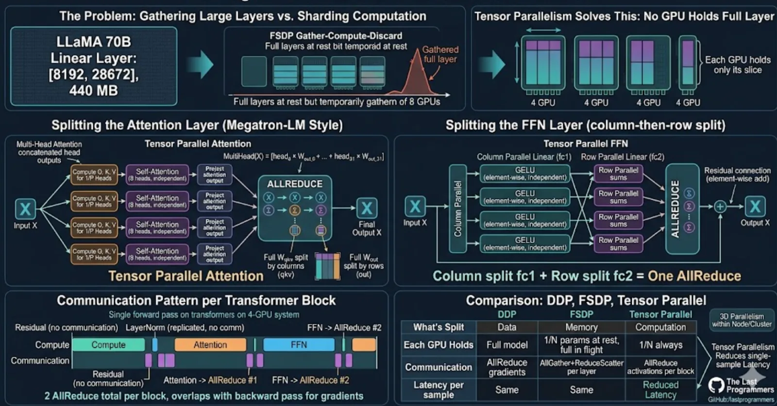
LLaMA 70B's largest linear layer: [8192, 28672] in bfloat16 = 440 MB. The full attention QKV projection + output + FFN for one layer: ~2.5 GB. With activations for a reasonable batch size: 5–10 GB per layer.

FSDP shards memory at rest, but during computation, every GPU temporarily gathers the full layer parameters (via AllGather). With 8 GPUs and a 70B model, each GPU still materializes the full layer during compute. The AllGather just moves the memory problem from "at rest" to "in flight."

Tensor parallelism solves this: no GPU ever holds the full layer. Each GPU holds and computes with only its slice.

The Core Idea

Instead of:

• One GPU does the full matrix multiply: Y = X × W where W is [4096 × 16384]

We split W across 4 GPUs:

• GPU 0 computes: Y_0 = X × W_0 where W_0 is [4096 × 4096]

• GPU 1 computes: Y_1 = X × W_1 where W_1 is [4096 × 4096]

• GPU 2 computes: Y_2 = X × W_2 where W_2 is [4096 × 4096]

• GPU 3 computes: Y_3 = X × W_3 where W_3 is [4096 × 4096]

Then combine the results (how depends on the split direction).

The key constraint: we must split in a way that produces the mathematically correct result with minimal communication.

Splitting the Attention Layer

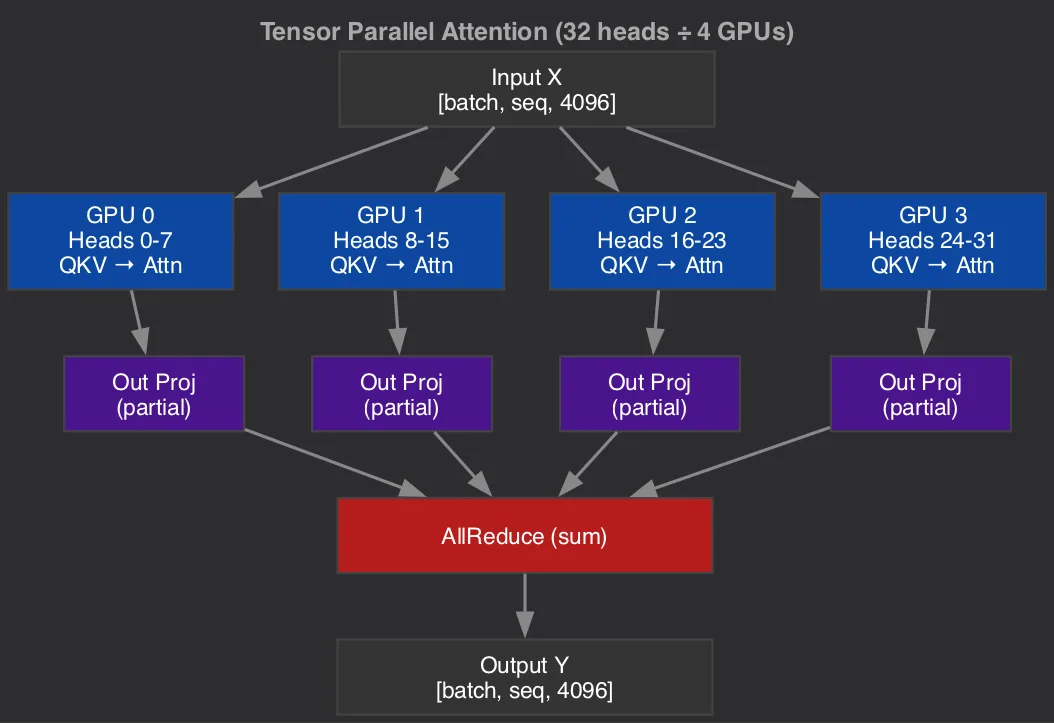
Multi-head attention is naturally parallelizable — the heads are independent.

With 32 attention heads and 4 GPUs, each GPU handles 8 heads:

Each GPU:

1. Computes Q, K, V for its heads only (1/P of the full QKV projection)

2. Runs self-attention independently (heads don't interact)

3. Projects its attention output through its slice of the output projection

4. AllReduce to sum partial results into the final output

The QKV weight matrix splits by columns (each GPU gets columns for its heads):

Full W_qkv: [4096, 3 × 4096] → each GPU gets [4096, 3 × 1024]
Full W_out: [4096, 4096]      → each GPU gets [1024, 4096] (split by rows)

Why This Works

Multi-head attention concatenates head outputs then projects:

MultiHead(X) = Concat(head_0, head_1, ..., head_31) × W_out
             = [head_0 × W_out_0 + head_1 × W_out_1 + ... + head_31 × W_out_31]

This is a sum of independent terms — exactly what AllReduce computes. Each GPU computes its terms, AllReduce sums them. Mathematically identical to computing all 32 heads on one GPU.

Splitting the FFN Layer

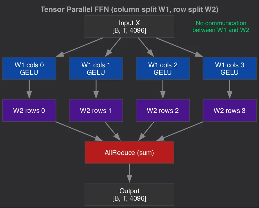
The feed-forward network: FFN(x) = GELU(x × W1) × W2

Where W1: [4096, 16384] and W2: [16384, 4096].

Split W1 by columns, W2 by rows:

Why column split on W1, row split on W2?

W1 column split: X × [W1_col0 | W1_col1 | ...] = [X×W1_col0 | X×W1_col1 | ...]

Each GPU gets an independent chunk of the hidden dimension. GELU is element-wise, so it applies independently to each chunk. No communication needed between W1 and W2.

W2 row split: The row split means each GPU's W2 slice expects only its chunk of the hidden dimension (which it already has from W1). The outputs are partial sums of the final result → AllReduce sums them.

The key insight: column-split first layer + row-split second layer = one AllReduce for the entire FFN. This is Megatron-LM's core contribution.

Communication Pattern per Transformer Block

A full transformer block with tensor parallelism requires only two AllReduce operations:

Input X
  │
  ├── LayerNorm (replicated, no communication)
  │
  ├── Attention (split by heads)
  │     └── AllReduce #1 (after output projection)
  │
  ├── Residual connection (element-wise add, no communication)
  │
  ├── LayerNorm (replicated, no communication)
  │
  ├── FFN (column split W1, row split W2)
  │     └── AllReduce #2 (after W2)
  │
  └── Residual connection (element-wise add, no communication)
  │
Output X

For a model with L layers: 2L AllReduce calls total. Each AllReduce moves batch × seq_len × embed_dim × sizeof(dtype) bytes.

For LLaMA 70B (80 layers, embed_dim=8192, bf16, seq_len=4096, batch=1):

• Per AllReduce: 4096 × 8192 × 2 bytes = 64 MB

• Total per forward pass: 160 × 64 MB = ~10 GB

Over 8 GPUs with NVLink (900 GB/s): ~11ms total communication. The compute time for 80 transformer layers dwarfs this.

Implementation Sketch

class ColumnParallelLinear(nn.Module):
    """Split weight matrix by columns across GPUs."""

    def __init__(self, in_features, out_features, world_size, rank):
        super().__init__()
        assert out_features % world_size == 0
        self.local_out = out_features // world_size
        self.weight = nn.Parameter(torch.empty(self.local_out, in_features))
        self.bias = nn.Parameter(torch.empty(self.local_out))

    def forward(self, x):
        # Each GPU computes its slice of the output
        return F.linear(x, self.weight, self.bias)


class RowParallelLinear(nn.Module):
    """Split weight matrix by rows across GPUs. AllReduces the output."""

    def __init__(self, in_features, out_features, world_size, rank):
        super().__init__()
        assert in_features % world_size == 0
        self.local_in = in_features // world_size
        self.weight = nn.Parameter(torch.empty(out_features, self.local_in))
        self.bias = nn.Parameter(torch.empty(out_features))

    def forward(self, x):
        # Each GPU computes a partial result
        local_out = F.linear(x, self.weight)
        # Sum across all GPUs
        dist.all_reduce(local_out, op=dist.ReduceOp.SUM)
        return local_out + self.bias


class TensorParallelAttention(nn.Module):
    def __init__(self, config, world_size, rank):
        super().__init__()
        assert config.n_heads % world_size == 0
        self.local_heads = config.n_heads // world_size
        self.head_dim = config.embed_dim // config.n_heads

        # Column parallel: each GPU gets QKV for its heads
        local_dim = self.local_heads * self.head_dim
        self.qkv = ColumnParallelLinear(config.embed_dim, 3 * local_dim, world_size, rank)

        # Row parallel: output projection, followed by AllReduce
        self.out_proj = RowParallelLinear(local_dim, config.embed_dim, world_size, rank)

    def forward(self, x):
        B, T, C = x.shape
        qkv = self.qkv(x)
        q, k, v = qkv.split(self.local_heads * self.head_dim, dim=-1)
        # ... attention computation with local heads only ...
        out = self.out_proj(attn_output)  # includes AllReduce
        return out


class TensorParallelFFN(nn.Module):
    def __init__(self, config, world_size, rank):
        super().__init__()
        # Column parallel on first layer
        self.fc1 = ColumnParallelLinear(config.embed_dim, 4 * config.embed_dim, world_size, rank)
        # Row parallel on second layer (includes AllReduce)
        self.fc2 = RowParallelLinear(4 * config.embed_dim // world_size, config.embed_dim, world_size, rank)

    def forward(self, x):
        x = F.gelu(self.fc1(x))  # each GPU has its slice
        x = self.fc2(x)          # AllReduce happens here
        return x

Tensor Parallelism vs Data Parallelism vs FSDP

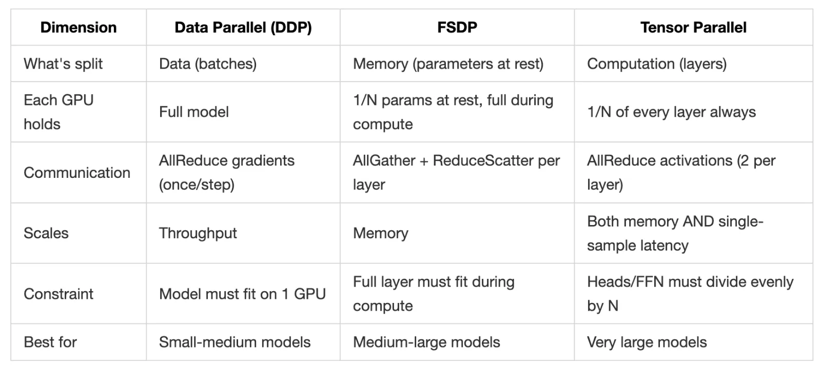
The key difference: tensor parallelism reduces latency for a single sample. DDP and FSDP both compute each sample on one GPU — more GPUs = more throughput but same per-sample latency. Tensor parallelism spreads one sample's computation across GPUs — more GPUs = lower latency AND lower per-GPU memory.

Combining All Three (3D Parallelism)

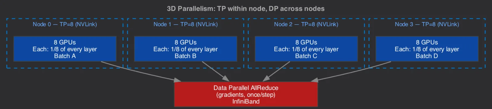
Production systems at scale use all three simultaneously. This is how GPT-4, LLaMA 405B, etc. are trained:

• Tensor parallel within a node (8 GPUs, NVLink at 900 GB/s)

• Data parallel / FSDP across nodes (slower network, but less frequent communication)

• Pipeline parallel (optional) — split layers across nodes for additional memory savings

Going Multi-Node: Tensor Parallelism in a Cluster

Tensor parallelism happens within a node (NVLink). But real training at frontier scale spans hundreds of nodes. This is where the 3D parallelism diagram above becomes concrete.

Why TP Stays Within a Node

TP requires 2 AllReduces per transformer block per forward pass. For LLaMA 70B (80 layers):

• 160 AllReduces per forward pass

• Each moves batch × seq_len × embed_dim × 2 bytes = e.g., 4 × 4096 × 8192 × 2 = 256 MB

• Total: 160 × 256 MB = 40 GB per forward pass

Over NVLink (900 GB/s): 44ms — hidden behind compute. Over InfiniBand (400 GB/s): 100ms — starts to dominate. Over ethernet (25 GB/s): 1600ms — completely unusable.

The rule: TP within NVLink distance, DP/FSDP across nodes.

Multi-Node Launch: TP + DP

# 4 nodes × 8 GPUs = 32 GPUs total
# TP=8 within each node, DP=4 across nodes

torchrun \
  --nnodes=4 \
  --nproc_per_node=8 \
  --rdzv_endpoint=$MASTER:29500 \
  train.py --tp_size=8 --dp_size=4

The system creates two overlapping communication groups — each GPU belongs to one TP group and one DP group:

32 GPUs across 4 nodes:

TP groups (communicate every layer, need NVLink):
  [GPU 0,1,2,3,4,5,6,7]      ← Node 0: these 8 GPUs split every layer
  [GPU 8,9,10,11,12,13,14,15] ← Node 1: independent copy of the model
  [GPU 16,...,23]              ← Node 2: independent copy
  [GPU 24,...,31]              ← Node 3: independent copy

DP groups (communicate once/step, tolerate InfiniBand):
  [GPU 0, 8, 16, 24]   ← "slice 0" across all nodes — same model shard, different data
  [GPU 1, 9, 17, 25]   ← "slice 1" across all nodes
  ...
  [GPU 7, 15, 23, 31]  ← "slice 7" across all nodes

Each TP group works together on every forward pass (fast, NVLink). Each DP group synchronizes gradients once per step (slower, InfiniBand — but infrequent). The key insight: high-frequency communication stays within the fast network; low-frequency communication crosses the slow network.

The Communication Pattern in Practice

One training step on 4 nodes × 8 GPUs (TP=8, DP=4):

1. Each node has the same model sharded across 8 GPUs (TP)
2. Each node processes a different batch of data

Forward pass (within each node):
  Layer 0: AllReduce activations across 8 GPUs (NVLink) × 2
  Layer 1: AllReduce activations across 8 GPUs (NVLink) × 2
  ...
  Layer 79: AllReduce activations × 2

Backward pass (within each node):
  Same AllReduces in reverse for gradient computation

Gradient sync (across nodes):
  AllReduce each GPU's gradients with its DP peers
  GPU 0 ↔ GPU 8 ↔ GPU 16 ↔ GPU 24 (InfiniBand)
  GPU 1 ↔ GPU 9 ↔ GPU 17 ↔ GPU 25
  ...
  (overlapped with backward computation of earlier layers)

Cross-node traffic is limited to the gradient AllReduce — exactly like DDP. The expensive per-layer communication stays within the fast NVLink domain.

Adding Pipeline Parallelism for Deeper Models

At extreme scale (405B+), even 3D parallelism isn't enough. Pipeline parallelism splits layers across nodes:

Node 0 (TP=8): Layers 0-19   (compute in parallel across 8 GPUs)
Node 1 (TP=8): Layers 20-39
Node 2 (TP=8): Layers 40-59
Node 3 (TP=8): Layers 60-79

Data flows: Node 0 → Node 1 → Node 2 → Node 3 (pipeline)
Each node only stores 1/4 of the layers

This introduces pipeline bubbles (GPUs idle while waiting for activations from the previous stage), but micro-batching minimizes them. The 1F1B (one-forward-one-backward) schedule keeps pipeline utilization at ~85-90%.

LLaMA 405B training uses: TP=8 (within node) × PP=4 (across 4 nodes) × DP=128 (across 128 such pipeline groups) = 4,096 GPUs.

Fault Tolerance at Scale

With 4,096 GPUs across 512 nodes, hardware failures happen daily. The standard approach:

1. Periodic checkpointing every 5-15 minutes
   - Each TP group saves its sharded state
   - Asynchronous checkpoint to shared storage (don't block training)

2. Health monitoring
   - NCCL watchdog: detect hung collectives (GPU failure mid-communication)
   - Heartbeat between nodes: detect network partition

3. Recovery
   - Kill the job
   - Replace the failed node (or reassign work to spare nodes)
   - Resume from last checkpoint
   - Lost work: 5-15 minutes × $cost_per_minute

4. Spare nodes
   - Keep 5-10% spare GPUs in the allocation
   - Automatic failover: re-form process groups with spares

At Meta's scale (16K GPUs for LLaMA 3 training), they reported ~3% of wall-clock time lost to failures/recovery. The infrastructure cost of frequent checkpointing is far lower than the cost of losing hours of training.

Running This On Your MacBook?

Tensor parallelism requires multiple GPUs that can communicate synchronously during a single forward pass. On a MacBook:

• You can't run tensor parallelism meaningfully (only one GPU)

• The code still runs in "TP=1" mode — functionally identical to the original model.py

• Testing: simulate on CPU with gloo backend and world_size > 1

class TransformerBlock(nn.Module):
    def __init__(self, config, world_size=1, rank=0):
        super().__init__()
        if world_size > 1:
            self.attn = TensorParallelAttention(config, world_size, rank)
            self.ff = TensorParallelFFN(config, world_size, rank)
        else:
            self.attn = CausalSelfAttention(config)  # original single-GPU code
            self.ff = FeedForward(config)

The MacBook is your development/debugging environment. Multi-GPU cloud instances are where tensor parallelism actually accelerates training.

Key Takeaways

1. Tensor parallelism splits computation, not data. Every GPU works on the same input but computes a different slice of the layer. This reduces both memory and latency per sample.

2. Attention is naturally parallel by heads. Multi-head attention was designed this way — heads are independent. Splitting across GPUs requires zero architectural changes.

3. Column-then-row split eliminates mid-layer communication. Megatron-LM's insight: split the first linear by columns and second by rows → one AllReduce for the entire FFN. Minimal communication for maximal parallelism.

4. Requires fast interconnect. Every transformer block needs 2 AllReduces during a single forward pass. With slow interconnect (ethernet), the communication dominates. Tensor parallelism only makes sense within a node (NVLink) or on InfiniBand clusters.

5. Production combines all three. Tensor parallel (within node) + Data parallel (across nodes) + FSDP (memory efficiency) = 3D parallelism. This is how every frontier model is trained.

Next: disaggregated inference — separating prefill and decode onto dedicated hardware pools for efficient serving at scale.

Full code: github.com/the-last-programmers/gpt-from-scratch